Association Analysis
Handout 07
Date: 2022-11-13
Topic: Simple Linear Regression
Literature
Handout
Ismay & Kim (2022) Chapter 5
Association Analysis
Association Analysis is a core topic in statistical analysis. It
involves measuring and modelling the relationship between variables in a
dataset.
See Ismay & Kim,
Chapter 5, Introduction.
Regression and Classification
In modelling association between a response variable (Y) and an
explanatory variable (X) distinction is made between a situation in
which the Y-variable is numeric and in which it is categorical. When the
Y-variable is numeric, it is called a regression
problem, otherwise it is called a classification
problem.
This chapter focusses on linear regression models with one X-variable:
simple linear regression. Multiple regression analysis involves more
than one X variable.
Example 1: HousePrices in Berlin district Spandau
This examples uses information about houses for sale in the Spandau district in Berlin in November 2019.
Table 7.1
First Six Observations Houses for Sale Berlin
library(tidyverse)
library(scales)
spandau <- read_csv("datafiles/forsale_berlin_spandau.csv")

head(spandau)
Figure 7.1
Scatterplot PRICE~AREA Houses for Sale, Berlin Spandau
#graphing with scatterplot
spandau %>%  ggplot(aes(x=AREA, y = PRICE)) +
  geom_point()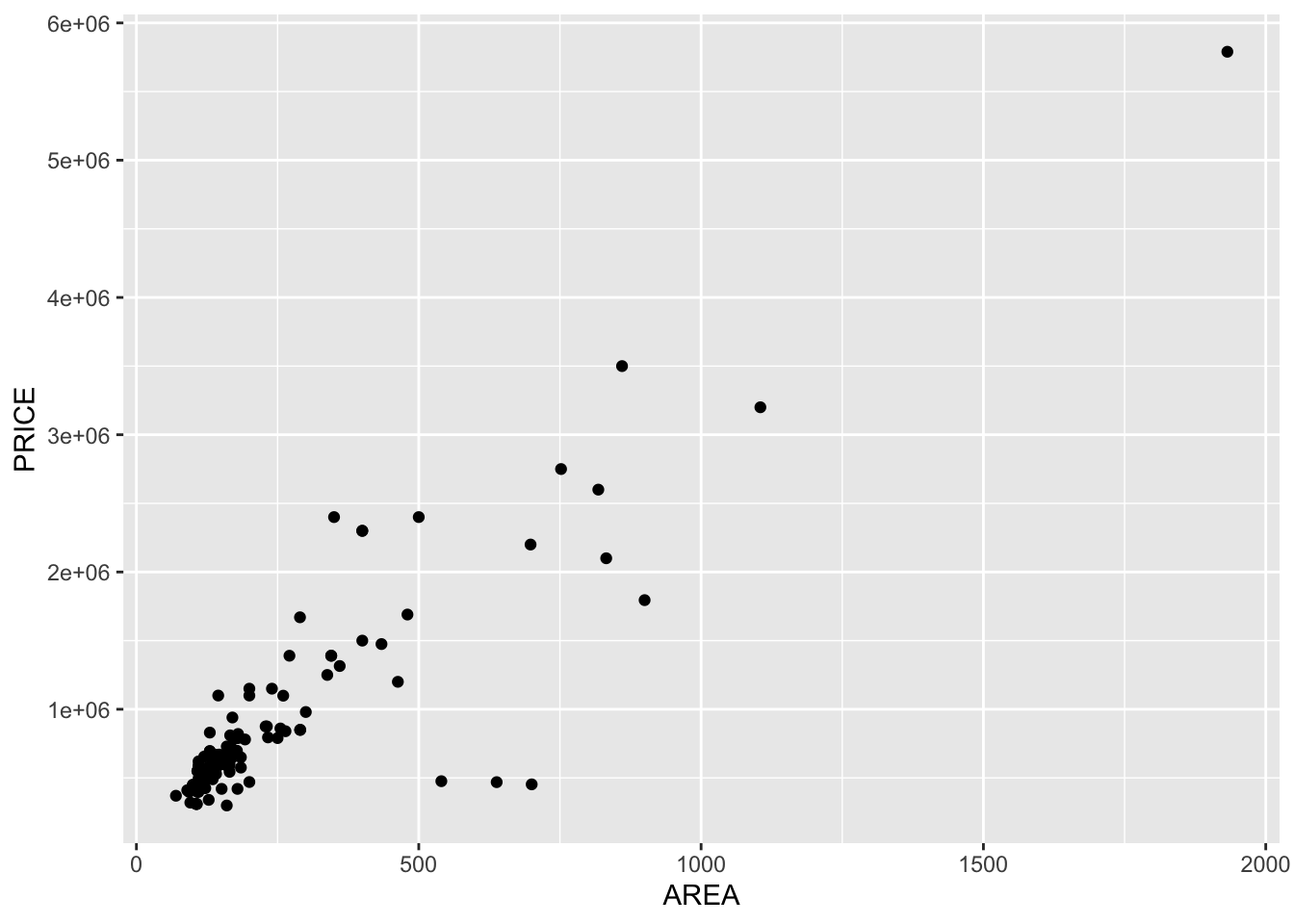
Figure 7.1 shows a positive linear correlation between the two
variables.
To measure the strongness of this relationship, the correlation
coefficient is used; see for instance this
website.
And see Rumsey, pp. 113-120 (forget the formulas).
The correlationcoefficient can be calculated with the
cor()-function.
cor(spandau$AREA, spandau$PRICE) = 0.881.
This indicates a strong positive linear relationship betwee AREA and
PRICE.
It does not indicate a causal
relationship between the two variables. Statistics can not do that;
statistics can support an assumed causal relationship between
variables.
In this example the assued relationship is unidirectional AREA —>
PRICE. In other words, AREA is the independent (explanatory) variable,
PRICE is the dependent (response) variable.
The next stap is modelling the relationship with a linear regression model.
Linear models
In general the equation of a straight line is: Y = \(\beta_{0}\) + \(\beta_{1}\)X
with \(\beta_{0}\) the intercept and
\(\beta_{1}\) the slope.
The intercept is the value where the line intersects the Y-axis.
The slope is the increase of Y as X increases by one unit.
Best Fitting Regression Line Criterion
The most used method to model a linear relationship: Ordinary Least
Square (OLS) Regression.
In R the lm() function is used to estimate a linear regression model
based on this criterion.
Table 7.2 Output Linear Model Summary
library(scales)
linmod <- lm(PRICE ~ AREA, data = spandau)
linmod_tabel <- summary(linmod)
summary(linmod)
##
## Call:
## lm(formula = PRICE ~ AREA, data = spandau)
##
## Residuals:
## Min 1Q Median 3Q Max
## -1674111 -87531 -19185 81175 1216656
##
## Coefficients:
## Estimate Std. Error t value Pr(>|t|)
## (Intercept) 239576.6 47124.3 5.084 0.00000142 ***
## AREA 2696.5 134.2 20.092 < 0.0000000000000002 ***
## ---
## Signif. codes: 0 '***' 0.001 '**' 0.01 '*' 0.05 '.' 0.1 ' ' 1
##
## Residual standard error: 362500 on 117 degrees of freedom
## Multiple R-squared: 0.7753, Adjusted R-squared: 0.7734
## F-statistic: 403.7 on 1 and 117 DF, p-value: < 0.00000000000000022Interpretation of the Output
The equation of estimated regression line is:
\(\hat{PRICE}\) = 239,577 + 2,696 \(\times AREA\)
The ‘hat’-symbol is used for model values.
The slope (2,696) gives the average increase of the model PRICE if the
AREA increase 1 m2.
The R-squared value (R2 = 0.775) in a simple linear
regression model, is the correlation coefficient squared.
Interpretation R2: the proportion of the
variation in the Y-variable that is explained by the
variation in the X-variable.
The actual values are scattered around the regression line.
The Residual Standard Error (RSE = 362,510) measures this variation
around the regression line.