Association Analysis (2)

Handout 08
Date: 2022-11-20
Topic: Association Analysis

Literature
Handout
Ismay & Kim (2022) Chapter 5 and 6

Association analysis

In many case data analysis is about analyzing association between variables: measuring the strength of a relationship, testing if the relationship is significant (or can be attributed to chance because the relationship is measured using a random sample), describing the relationship with a mathematical equation.
The objective of this kind of analysis can be predicting or estimating an output based on one or more inputs or just to examine the relationships between different variables and the structure of the data. In this lesson, the emphasis is on the former.

When it is about predicting and estimating there are one response (dependent) variable (the Y-variable) and one or more explanatory (independent) variables (X variables). Problems with a categorical response variable are referred to as classification problems, while those involving a numeric response as regression problems.

Relationships between two categorical variables

Common ways to examine relationships between two categorical variables:

Graphical: clustered bar chart; stacked bar chart
Descriptive statistics: cross tables
Metric to measure the strength of the relation:
- phi coefficent, in case of two binary variables
- Cramer’s V
  see: http://groups.chass.utoronto.ca/pol242/Labs/LM-3A/LM-3A_content.htm and use
Hypotheses testing:
- tests on difference between proportions
- chi-square tests a test to test if two categorical variables are independent

Example: PPD LONDON, association between OLD/NEW and LEASEHOLD/FREEHOLD
Research sub question: is there a dependency between the variables OLD/NEW and LEASEHOLD/FREEHOLD for properties in London?
The question is answered based on the properties sold in January 2019.

Table 1
Houses sold in London in January 2019,
divided by TYPE and FREEHOLD/LEASHOLD

library(openxlsx)
library(tidyverse)
library(flextable)
library(sjstats)
ppd <- read.xlsx("datafiles/HP_LONDON_JAN19.xlsx")
tab01 <- xtabs(~ TYPE + DURATION, data = ppd)
tab01.01 <- ppd %>% 
  group_by(TYPE, DURATION) %>% 
  summarize(COUNT= n()) %>% 
  spread(DURATION, COUNT) %>% 
  ungroup() %>% 
  mutate(TYPE = factor(TYPE))
levels(tab01.01$TYPE) <- list(TERRACED = "T", FLAT = "F",
                              DETACHED = "D", `SEMI-DETACHED` = "S")

ft <- flextable(tab01.01) %>% 
  autofit()
ft

TYPE	F	L
DETACHED	35	2
FLAT	7	775
SEMI-DETACHED	121	4
TERRACED	420	22

#phi(tab01)
#cramer(tab01)
#chisq.test(tab01)

Note. As can be seen in this table the distribution over the Freehold and Leashold categories differ for the different types. The question is, if the association between the two variables is significant.
The strength of the relationship can be measured by Cramer’s V, this metric has a value of 0.949 in this case. This means there is a very strong relationship between TYPE and FREEHOLD/LEASHOLD; if the type is known good predictions can be made for the FREEHOLD/LEASEHOLD category.

Example: crime incidents in 2017 in Washington, D.C.
The file Crime_Incidents_in_2017.csv (source: http://us-city.census.okfn.org/) contains information about crimes in Washington D.C. in 2017.
To analyse if there is a relationship between the variables METHOD, a categorical variable with free unique values (GUN, KNIFE and OTHERS), and SHIFT a categorical variable with three unique values (DAY, EVENING, MIDNIGHT) a contingency table has been created.

Figure 1
Crimes in Washington D.C. in 2017

crimes <- readr::read_csv("datafiles/Crime_incidents_In_2017.csv") %>%
  filter(METHOD != "OTHERS")
tab02 <- xtabs(~ METHOD+SHIFT, data = crimes)
crimes01 <- crimes %>%
  filter(METHOD != "OTHERS") %>% 
  group_by(METHOD, SHIFT) %>% 
  summarize(COUNT = n()) %>% 
  spread(SHIFT, COUNT)

ft <- flextable(crimes01) %>% autofit()  
#ft <- set_caption(ft, x)

ggplot(crimes, aes(x=SHIFT, group = METHOD, fill = METHOD)) +
  geom_bar(position = "dodge") +
  xlab(NULL) +
  theme_light()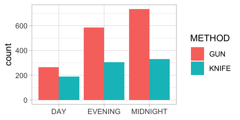

cram02 <- sjstats::cramer(tab02)
chisq02 <- chisq.test(crimes01[,2:4])
chi02 <- scales::comma(chisq02$statistic, accuracy = .01)
p02 <- ifelse(chisq02$p.value<.001, "< .001", paste("=", comma(chisq02$p.value, accuracy=.001)))

Table 2
Crimes in Washington D.C. in 2017

ft

METHOD	DAY	EVENING	MIDNIGHT
GUN	266	585	734
KNIFE	188	306	330

In this example Cramer’s V equals 0.08. The relationship between the two variables is very weak, although it is significant, chisquare(2) = 15.29, p < .001.

Relationship between categorical and numeric variable

Common ways to examine relationships between two categorical variables:

Graphical: side-by-side boxplots, side-by-side histograms, multiple density curves
Tabulation: five number summary/ descriptive statistis per category in one table
Hypotheses testing:
- t test on difference between means
- Wilcoxon ranksumtest (also called Mann Whitney U-test) (also applicable in the case of small samples)

Example: comparison airpollution between Amsterdam and Rotterdam
A comparison of the difference between airpollution caused by PM10 in Amsterdam, location Einsteinweg and Rotterdam, location Statenweg. The comparison is based on the figures from 2018 as reported on the RIVM website.

library(scales)
airq <-
  read_csv("/Users/R/10Rprojects/AirQuality/Output/oaq2018_nl_majorcities.csv")  %>%    
    mutate(DATE = lubridate::date(lubridate::ymd_hms(tijdstip))) %>% 
    filter(component == "PM10",                                                                    locatie %in% c("Amsterdam-Einsteinweg", "Rotterdam-Statenweg"),
           waarde >= 0,
           DATE >= "2018-01-01", DATE <= "2018-12-31") %>% 
    select(DATE, TIME = tijdstip, CITY = city, LOCATION = locatie, COMPONENT = component, VALUE = waarde, AQI = LKI)

airq_daily <- airq %>% 
  group_by(DATE, CITY, LOCATION) %>% 
    summarize(AVG_VALUE = mean(VALUE, na.rm = TRUE))

airq_table <- airq_daily %>% 
  group_by(CITY, LOCATION) %>% 
  summarize(COUNT = n(),
            MINIMUM = min(AVG_VALUE),
            Q1 = quantile(AVG_VALUE, .25),
            MEDIAN = median(AVG_VALUE),
            Q3 = quantile(AVG_VALUE, .75),
            MAXIMUM = max(AVG_VALUE),
            AVERAGE = round(mean(AVG_VALUE), 2),
            SD = round(sd(AVG_VALUE), 2)) 

M_ams <- comma(mean(airq_daily$AVG_VALUE[airq_daily$CITY == "Amsterdam"]), accuracy = .1)
M_rot <- comma(mean(airq_daily$AVG_VALUE[airq_daily$CITY == "Rotterdam"]), accuracy = .1)
SD_ams <- comma(sd(airq_daily$AVG_VALUE[airq_daily$CITY == "Amsterdam"]), accuracy = .1)
SD_rot <- comma(sd(airq_daily$AVG_VALUE[airq_daily$CITY == "Rotterdam"]), accuracy = .1)

airq_daily_wide <- airq_daily %>% 
  select(DATE, CITY, AVG_VALUE) %>% 
  spread(CITY, AVG_VALUE) %>% 
  na.omit()

ttest <- t.test(airq_daily_wide$Amsterdam,
                airq_daily_wide$Rotterdam,
                paired = TRUE)
tvalue <- comma(ttest$statistic, accuracy=.001)
pvalue <- ifelse(ttest$p.value < .001, "< .001", 
                 paste("=", comma(ttest$p.value, accuracy=.001)))
dfvalue <- round(ttest$parameter)

Figure 2
Daily average PM10 levels in 2018 on a location in Amsterdam and a location in Rotterdam

ggplot(airq_daily, aes(x=LOCATION, y = AVG_VALUE)) +
  geom_boxplot() +
  coord_flip() +
  xlab(NULL) +
  ylab("PM10 level") +
  theme_minimal()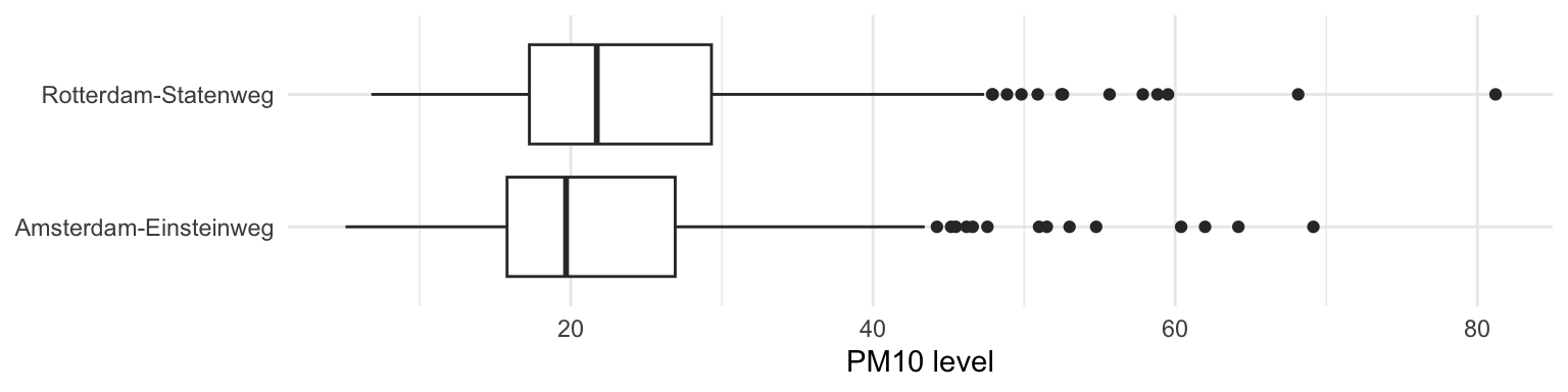

Note. Overall air quality in Rotterdam is worse than in Amsterdam.

Table 3
Summary statistics daily PM10 levels

flextable(airq_table) %>% autofit()

CITY	LOCATION	COUNT	MINIMUM	Q1	MEDIAN	Q3	MAXIMUM	AVERAGE	SD
Amsterdam	Amsterdam-Einsteinweg	363	5.086957	15.78333	19.68750	26.91042	69.14583	22.45	10.05
Rotterdam	Rotterdam-Statenweg	365	6.800000	17.25833	21.72083	29.31250	81.20417	24.32	10.55

A paired t-test is used to investigate whether the daily average values in Amsterdam-Einsteinweg differ from these in Rotteram-Statenweg. Based on this test it can be concluded that the difference between the daily values in Amsterdam (M = 22.5, SD = 10.0) and Rotterdam (M = 24.3, SD = 10.5) is significant, t(362) = -8.847, p < .001.

Relationship between two numerical variables

Common ways to examine relationships between two numerical variables:

Graphs per variable in order to verify if there are any outliers (boxplots / histograms).
Table: summary statistics per variable; verify if there are missing data.
Graphical: Scatterplot to graph the relationship between the two variables. Verify if the graph supports that there exists a linear relationship and examine if there are outliers.
Measure of linear association: correlation coefficient.
Notice: statistical association is not the same as a causal relation!!
Describing the relationship using a mathematical model: linear regression analysis.

Example: Dutch cars

The RDWregr.xlsx file contains data of a number of vehicles including the mass and the selling price.¹ It may be assumed that there is a relationship between mass and selling price.
1. Generate a table with the most important statistics concerning the two variables.
2. Create boxplots.
3. Create a scatterplot; examine the outliers; does the graph support the assumption about a relationship between mass and selling price.
4. The strength of the relationship can be measured with the correlation coefficient r (see below); what’s the value of r (use Excel function correl() )?
5. The relationship can be described by a mathematical equation; right click on the dots in the graph and choose the option to plot the best fitting line and display the equation on chart.

Correlation coefficient

The correlation coefficient r is a measure for the strength of a linear relationship between two variables. More about how to interpret a correlation coefficient can be found on this website .

Significant correlation

Even when there is no correlation between two variables the correlation coefficient calculated based on a sample will not be 0. That’s why it is quite common to use a significance test to test whether the r value differs significantly from 0. More about this test can be found here.

Least square regression

Video.
In Excel, the equation of the OLS (Ordinary Least Squares) regression line can be found in different ways:
- Plotting the regression line and its equation in the scatterplot.
- Using menu choice: data/data analysis/regression.
- Using formulas to calculate the intercept (formula: intercept) and the slope (formula: slope) of the regression line.

MS Excel regression output

Figure 3 shows the MS Excel regression output for the Dutch car examples (see abve).

Figure 3
Regression output created with 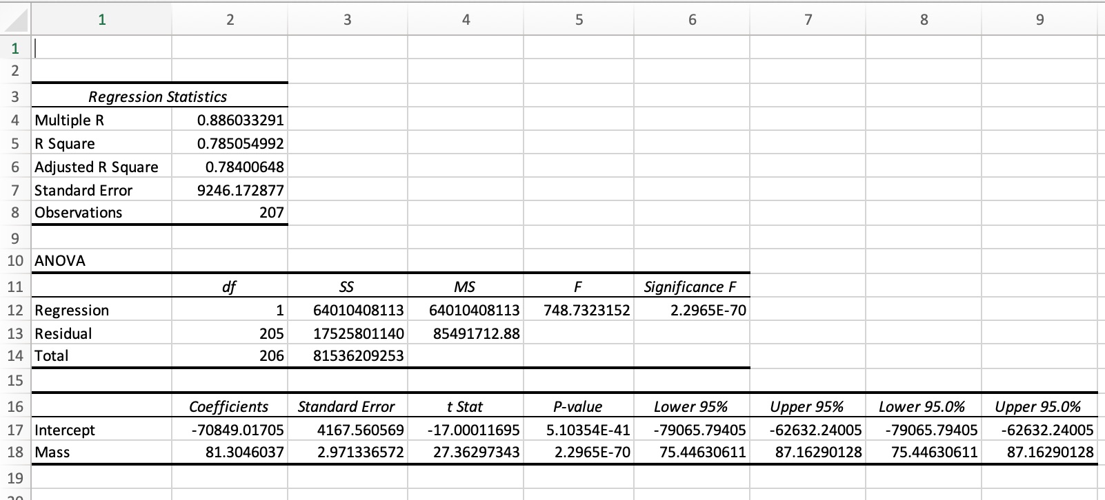MS Excel Note. Menu choice in Excel: data/Data Analysis/Regression. To use this option, first activate the Data Analysis Toolpack in MS Excel.

The regression model in the example output in figure 4 can be described by the equation:
CATALOG PRICE = -70,849 + 81.30 x MASS, where
MASS is the mass of the car in kg, and
CATALOG PRICE is the catalog price in euro.

Figure 4
Regression output RDW example

rdw <- openxlsx::read.xlsx("datafiles/RDWregr.xlsx")
rdw_linmod <- lm(Catalog_price ~ Mass, data = rdw)
summary(rdw_linmod)


Call:
lm(formula = Catalog_price ~ Mass, data = rdw)

Residuals:
   Min     1Q Median     3Q    Max 
-47701  -4551   -765   4342  50948 

Coefficients:
              Estimate Std. Error t value Pr(>|t|)    
(Intercept) -70849.017   4167.561  -17.00   <2e-16 ***
Mass            81.305      2.971   27.36   <2e-16 ***
---
Signif. codes:  0 '***' 0.001 '**' 0.01 '*' 0.05 '.' 0.1 ' ' 1

Residual standard error: 9246 on 205 degrees of freedom
Multiple R-squared:  0.7851,    Adjusted R-squared:  0.784 
F-statistic: 748.7 on 1 and 205 DF,  p-value: < 2.2e-16

It’s also possible to use functions from other packages. The ‘moderndive package’ comes, among others, with some functions to create output for a regression analysis.

Figure 5
Regression output RDW example using moderndive::

rdw <- openxlsx::read.xlsx("datafiles/RDWregr.xlsx")
rdw_linmod <- lm(Catalog_price ~ Mass, data = rdw)
moderndive::get_regression_table(rdw_linmod)

Assessing the regression model

After generating a regression model it is important to assess the model. This is done to judge whether the model fits the data and, in case of comparing models, which model fits the data best.

Coefficient of determination R²
In case of simple linear regression, i.e. with just one X-variable, the R2 value is the correlation coefficient squared. In a multiple regression setting it’s more complicated.

In general, the following equation holds: R² = \(\frac{variation\ of\ the\ model\ Yvalues\ around\ the\ mean\ Yvalue}{variation\ of\ the\ Yvalues\ around\ the\ mean\ Yvalue}\) = \(\frac{\Sigma(\widehat{Y} - \bar{Y})^{2}} {\Sigma(Y - \bar{Y})^{2}}\)

The denominator of this expression, \(\Sigma(Y - \bar{Y})^{2}\), measures the total variation in the Y-values around the mean Y-value, while the numerator, \(\Sigma(\widehat{Y} - \bar{Y})^{2}\), measures the variation of the model Y-values (the \(\widehat{Y}\)-values) around the mean Y-value. The latter is the variation in the Y-values that is explained by the regression model.
So R² measures the proportion of the variation in the Y-values that is explained by the regression model. In all cases: 0 <= R² <= 1.

The standard error of the estimate s_e
The standard error of the estimate is a metric for the spread around the regression line.
The value can be used to estimate the so-called margin of error if the model is used to predict a Y-value given the X-value(s). As a rule of thumb, the margin of error that should be taken in account when predicting a Y-value is 2xs_e.
So the smaller the s_e value the better the model can predict a Y-value.
To evaluate the value of s_e, it is compared with \(\bar{Y}\), commonly by dividing s_e by \(\bar{Y}\).

P-values of the coefficient(s)
The P-values of the model coefficients are used to determine whether the different X-variables are significant in the model. Most common interpretation: a P-value less than .05 indicates that the X-variable is significant. The test for which this P-value is calculated is:
H₀: \(\beta\) = 0
H_A: \(\beta\) <> 0, where \(\beta\) is the coefficient of the X-variable in question.
Not rejecting H₀ means the coefficient of the X-variable doesn’t differ significantly from 0, in other words Y doesn’t depend significantly on X.

Assessing the model in the RDW example

R² = .785, which means that 78.5% of the variation in catalog prices is explained by the variation in masses.
s_e = 9246; if the model is used to estimate the catalog price, based on the mass of a car, a margin of error of 18,492 (2 x s_e) should be taken in account. In other words, this model is not a very good model to predict catalog prices.
The regression coeeficient of the MASS variable (81.3) differs significantly from 0, p < .001. MASS is a significant variable.

Multiple linear regression, an example

The buyer of a new car has to pay a special tax. The heigth of this special tax depends on different factors. Aim of this example is to find a model with which the heigth of the special tax for a Toyota can be estimated, based on different characteristics of this car. For this reason a random sample from in the Netherlands registered Toyota’s has been drawn, reference date 2019-06-12; see file toyota_sample.csv.

Table 4
Toyota Sample, first 10 observations

library(tidyverse)
toyota <- read_csv("Datafiles/toyota_sample.csv")
graph01 <- ggplot(toyota, aes(x = SPECIAL_TAX)) +
  geom_histogram(fill = "royalblue")
graph02 <- ggplot(toyota, aes(x=CATALOG_PRICE, y =SPECIAL_TAX)) +
  geom_point(col = 'royalblue') +
  theme_minimal()

linmod00 <- lm(SPECIAL_TAX ~ CATALOG_PRICE, data = toyota)
linmod01 <- lm(SPECIAL_TAX ~ MASS, data = toyota)
linmod02 <- lm(SPECIAL_TAX ~ MASS+CATALOG_PRICE, data = toyota)

flextable::flextable(head(toyota, n=10)) %>% 
  fontsize(size=9, part="all") %>% autofit()

LICENSE_PLATE	BRAND	ECONOMY_LABEL	FUEL_DESCRIPTION	CILINDER_CONTENT	MASS	CATALOG_PRICE	SPECIAL_TAX
25ZGBP	TOYOTA	D	PETROL	1,598	1,320	24,800	5,808
SB674R	TOYOTA	A	ELECTRICITY	1,497	1,065	20,420	628
KV635K	TOYOTA	A	ELECTRICITY	1,497	1,060	20,222	519
1TPH61	TOYOTA	A	PETROL	998	945	16,063	629
31TNKR	TOYOTA	B	PETROL	1,298	1,000	16,941	3,185
89TBVX	TOYOTA	C	PETROL	1,298	995	17,430	3,682
36ZNZX	TOYOTA	A	PETROL	998	805	10,580	678
KJ092K	TOYOTA	A	ELECTRICITY	1,497	1,070	22,335	856
HH024S	TOYOTA	A	ELECTRICITY	1,798	1,310	31,445	667
JX218K	TOYOTA	B	PETROL	998	830	13,685	1,270

Data description

The sample contains almost 400 observations.

As a first analysis the correlation coefficients between some of the numeric variables has been calculated.

Table 5 Correlation matrix

cor(toyota[,c("CILINDER_CONTENT", "MASS", "CATALOG_PRICE", "SPECIAL_TAX")],
    use="complete.obs") %>% round(3)

                 CILINDER_CONTENT  MASS CATALOG_PRICE SPECIAL_TAX
CILINDER_CONTENT            1.000 0.937         0.847       0.531
MASS                        0.937 1.000         0.920       0.556
CATALOG_PRICE               0.847 0.920         1.000       0.644
SPECIAL_TAX                 0.531 0.556         0.644       1.000

As can be seen in Table 6 the variable SPECIAL_TAX has the highest correlation with CATALOG_PRICE. That’s why the first regression model is a simple linear regression model with CATALOG_PRICE as explanatory variable.

Figure 5
Scatterplot, SPECIAL_TAX in euro against CATALOG_PRICE in euro

graph02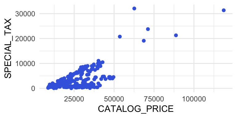

Simple linear models

A first model uses CATALOG_PRICE as explanatory variable.

Figure 6
Simple linear regression model with SPECIAL_TAX ~ CATALOG_PRICE

summary(linmod00)


Call:
lm(formula = SPECIAL_TAX ~ CATALOG_PRICE, data = toyota)

Residuals:
    Min      1Q  Median      3Q     Max 
-5202.1 -2457.3   -48.4  1552.8 21545.2 

Coefficients:
                Estimate Std. Error t value Pr(>|t|)    
(Intercept)   -2.721e+03  3.548e+02  -7.669 1.36e-13 ***
CATALOG_PRICE  2.114e-01  1.263e-02  16.734  < 2e-16 ***
---
Signif. codes:  0 '***' 0.001 '**' 0.01 '*' 0.05 '.' 0.1 ' ' 1

Residual standard error: 2839 on 395 degrees of freedom
  (3 observations deleted due to missingness)
Multiple R-squared:  0.4148,    Adjusted R-squared:  0.4134 
F-statistic:   280 on 1 and 395 DF,  p-value: < 2.2e-16

A second model uses MASS as explanatory variable.

Figure 7
Simple linear regression model with SPECIAL_TAX ~ MASS

summary(linmod01)


Call:
lm(formula = SPECIAL_TAX ~ MASS, data = toyota)

Residuals:
    Min      1Q  Median      3Q     Max 
-5453.7 -2541.8  -234.7  1467.7 26311.6 

Coefficients:
              Estimate Std. Error t value Pr(>|t|)    
(Intercept) -6396.8549   702.5876  -9.105   <2e-16 ***
MASS            7.6394     0.5753  13.279   <2e-16 ***
---
Signif. codes:  0 '***' 0.001 '**' 0.01 '*' 0.05 '.' 0.1 ' ' 1

Residual standard error: 3080 on 398 degrees of freedom
Multiple R-squared:  0.307, Adjusted R-squared:  0.3053 
F-statistic: 176.3 on 1 and 398 DF,  p-value: < 2.2e-16

Multiple linear model: SPECIAL_TAX ~ MASS + CATALOG_PRICE

In the next model two explanatory variables ares used: MASS and CATALOG_PRICE.

Figure 8
Multiple Linear Regression Model SPECIAL_TAX ~ CATALOG_PRICE + MASS

summary(linmod02)


Call:
lm(formula = SPECIAL_TAX ~ MASS + CATALOG_PRICE, data = toyota)

Residuals:
   Min     1Q Median     3Q    Max 
 -5166  -2266   -373   1370  20180 

Coefficients:
                Estimate Std. Error t value Pr(>|t|)    
(Intercept)   -628.91679  915.16671  -0.687   0.4924    
MASS            -3.33629    1.34651  -2.478   0.0136 *  
CATALOG_PRICE    0.28453    0.03207   8.873   <2e-16 ***
---
Signif. codes:  0 '***' 0.001 '**' 0.01 '*' 0.05 '.' 0.1 ' ' 1

Residual standard error: 2821 on 394 degrees of freedom
  (3 observations deleted due to missingness)
Multiple R-squared:  0.4238,    Adjusted R-squared:  0.4209 
F-statistic: 144.9 on 2 and 394 DF,  p-value: < 2.2e-16

Although this model uses two explanatory variables which are both moderately correlated with the response variable SPECIAL_TAX, the model is not much better than the simple linear models. The reason for this is that the two explanatory variables are highly correlated with each other. In general it is preferable to use explanatory variables which are not correlated to each other.

Multiple linear model: SPECIAL_TAX ~ CATALOG_PRICE + FUEL_DESCRIPTION

The next model makes use of a dummy variable ELECTRIC (1 = FUEL_DESCRPTION=“ELECTRICITY”, 0 = FUEL_DESCRPTION<>“ELECTRICITY”).

Figure 9
Scatterplot SPECIAL_TAX ~ ELECTRIC

toyota %>% ggplot(aes(x=ELECTRIC, y=SPECIAL_TAX)) +
  geom_point()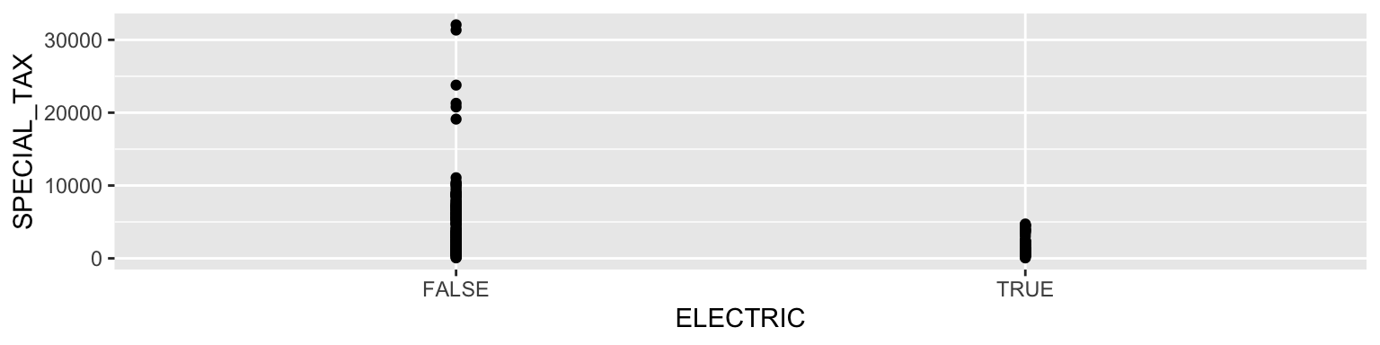

Figure 10
Multiple Regression Model with a Dummy Variable SPECIAL_TAX ~ CATALOG_PRICE + ELECTRIC

library(dplyr)
toyota<- toyota |> 
  mutate(ELECTRIC = ifelse(FUEL_DESCRIPTION == "ELECTRICITY", 1, 0))
linmod03 <- lm(SPECIAL_TAX ~ CATALOG_PRICE+ELECTRIC, data = toyota)
summary(linmod03)


Call:
lm(formula = SPECIAL_TAX ~ CATALOG_PRICE + ELECTRIC, data = toyota)

Residuals:
    Min      1Q  Median      3Q     Max 
-5431.3  -892.2  -217.6   801.3 16619.8 

Coefficients:
                Estimate Std. Error t value Pr(>|t|)    
(Intercept)   -1.965e+03  1.959e+02  -10.03   <2e-16 ***
CATALOG_PRICE  2.779e-01  7.255e-03   38.31   <2e-16 ***
ELECTRIC      -4.974e+03  1.637e+02  -30.39   <2e-16 ***
---
Signif. codes:  0 '***' 0.001 '**' 0.01 '*' 0.05 '.' 0.1 ' ' 1

Residual standard error: 1555 on 394 degrees of freedom
  (3 observations deleted due to missingness)
Multiple R-squared:  0.825, Adjusted R-squared:  0.8241 
F-statistic: 928.9 on 2 and 394 DF,  p-value: < 2.2e-16

Note. This model is really an improvement of the simple regression model with CATALOG_PRICE as the only explanatory variable.

In R it is possible to use a catagorical variable as explanatory variable in a regression analysis. In such a case, R transforms the catagorical variable in a number of dummies.
For instance, in the Toyota example the categorical variable FUEL_DESCRIPTION can be added as explanatory variable.
This variable has four unique values: PETROL, ELECTRICITY, DIESEL, LPG.
R creates three dummy variables, not four. After all, if the value of three of the four possible dummy variables is known, the fourth is known as well.

Figure 11
Multiple Regression Model with a Dummy Variable SPECIAL_TAX ~ CATALOG_PRICE + FUEL_DESCRIPTION

linmod04 <- lm(SPECIAL_TAX ~ CATALOG_PRICE+FUEL_DESCRIPTION, data = toyota)
summary(linmod04)


Call:
lm(formula = SPECIAL_TAX ~ CATALOG_PRICE + FUEL_DESCRIPTION, 
    data = toyota)

Residuals:
    Min      1Q  Median      3Q     Max 
-4868.7  -819.6  -220.4   945.8 17536.0 

Coefficients:
                              Estimate Std. Error t value Pr(>|t|)    
(Intercept)                  3.387e+02  5.520e+02   0.614    0.540    
CATALOG_PRICE                2.593e-01  8.267e-03  31.366  < 2e-16 ***
FUEL_DESCRIPTIONELECTRICITY -6.734e+03  4.261e+02 -15.803  < 2e-16 ***
FUEL_DESCRIPTIONLPG         -1.989e+03  1.571e+03  -1.266    0.206    
FUEL_DESCRIPTIONPETROL      -2.051e+03  4.608e+02  -4.451 1.12e-05 ***
---
Signif. codes:  0 '***' 0.001 '**' 0.01 '*' 0.05 '.' 0.1 ' ' 1

Residual standard error: 1520 on 392 degrees of freedom
  (3 observations deleted due to missingness)
Multiple R-squared:  0.8335,    Adjusted R-squared:  0.8318 
F-statistic: 490.5 on 4 and 392 DF,  p-value: < 2.2e-16

This model is not really an improvement compared with the former model.

The data set is not a random sample from all registered cars in the Netherlands; it is a random sample from registered cars from three brands, KIA, BMW and AUDI; because of didactic reasons, KIA PICANTO’s are excluded from the sample.↩︎